HSCP Mass Reconstruction
A summary of my Fermilab internship, not a paper. Three ways of turning a particle's ionization into a mass, tried on a simulated heavy gluino.
From July to October 2025 I was at Fermilab on the US-CMS PURSUE program, working with Dr. Emery Nibigira on the search for a heavy stable charged particle — something new and much heavier than a proton, which crosses the whole detector instead of decaying where it was made. A proton is about 1 GeV. The sample I worked on is a simulated gluino of 1800 GeV.
What the detector records
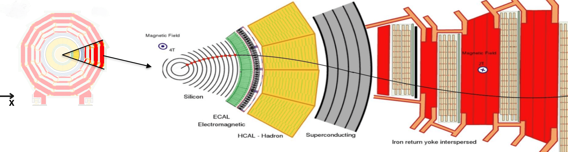
A charged particle crossing CMS leaves a hit in every silicon layer it passes, and the tracker reads two things off those hits: the momentum, and how much energy the particle gave up on the way, written dE/dx.
For almost everything the LHC makes, that second number tells you nothing. Those particles move so close to the speed of light that they all ionize about the same amount whatever they are, which is the bright horizontal band running across the plot below. Ionization only climbs once a particle slows down, which is why the familiar light species peel apart on the left where momentum is low. A gluino heavy enough to still be slow at high momentum would sit above the band, on its own. Momentum is mass times speed, so ionization and momentum together give you a mass, and that is the whole method.
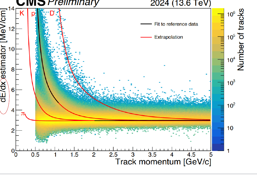
That plot is CMS's own, from 2024 collisions — the picture of the idea rather than my data.
Why you cannot just average
A track carries somewhere between ten and thirty hits. Most are small, and a few are enormous: a knock-on electron, or a glitch in the sensor. Here is every hit in the sample, peaking near 7 MeV/cm, with the circled tail running out past 20.
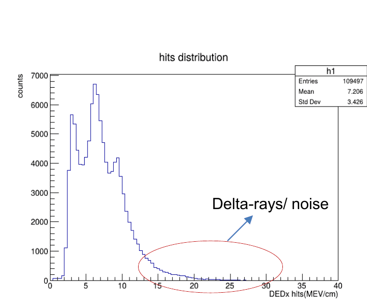
Average those and the tail drags the answer upward, the mass smears, and the search loses reach. So the problem is to collapse one track's hits into a single number that the wild ones do not own.
Three ways to do it
All three ran on the 2018 simulation of that gluino, no collision background, about 11,000 tracks after the isolated-track selection.
Harmonic-2 is CMS's baseline. Each hit is weighted by one over its ionization squared, so an enormous hit barely registers.
A 40% truncated mean throws away the highest 40% of the hits and averages what is left. Blunt, and it works.
A Landau fit, one per track. That lopsided shape has a name, so rather than averaging at all, fit the curve and take its most probable value. Fixed histogram bins wreck this when some tracks carry ten hits and others thirty, so I set the bin width from the track's own hits and started the fit at the tallest bin. Convergence went from 73% to 89.6%, at 0.44 ms per track on one core.
It still fails two ways. Around 0.2% of tracks come back with a negative peak, every one of them carrying a single hit far above the rest, and about 5% collapse to zero width, mostly tracks with four hits or fewer. Both should fall back to Harmonic-2, which I never got round to building.
Before any of this becomes a mass: narrower is better, and less tail is better. The core is 3.8 to 15 MeV/cm, the tail anything past 20.
| Estimator | Core width | Full width | Share above 20 MeV/cm |
|---|---|---|---|
| Harmonic-2 | 0.312 | 0.485 | 0.15% |
| 40% truncated mean | 0.296 | 0.492 | 0.14% |
| Landau fit | 0.336 | 0.492 | 0.35% |
Width is spread over centre, so smaller is sharper. The 40% cut edges out Harmonic-2 and stays just as quiet in the tail, while the Landau fit comes out slightly wider and lets more of the extreme through. None of that settles which gives the sharper mass peak, so I went and reconstructed the mass.
The masses
Mass comes out of ionization and momentum through two constants, K and C, fitted on known particles. I used one pair for all three estimators — K = 2.49, C = 3.18, from Harmonic-2 on this sample — which keeps the comparison honest about shape, but means only the blue histogram sits on a scale I trust. The other two are borrowing.
It is a thin slice: 7% of the NanoAOD survives the cuts, 558 events and about 1,100 tracks.
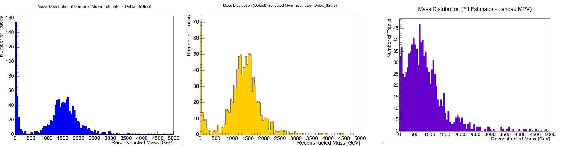
Blue is the peak to trust for where 1800 GeV falls. Yellow is the same tracks with the top hits dropped. Purple is the Landau fit, and it is a mess, with a small second bump near 1900 GeV.
I do not know what that bump is. Fits that should have been thrown out, a bad hit that should have been masked first, or something in the sample itself. On a borrowed calibration I would not claim the purple peak sits anywhere in particular. Giving the fit its own K and C and rejecting the bad fits is the check that would settle it.
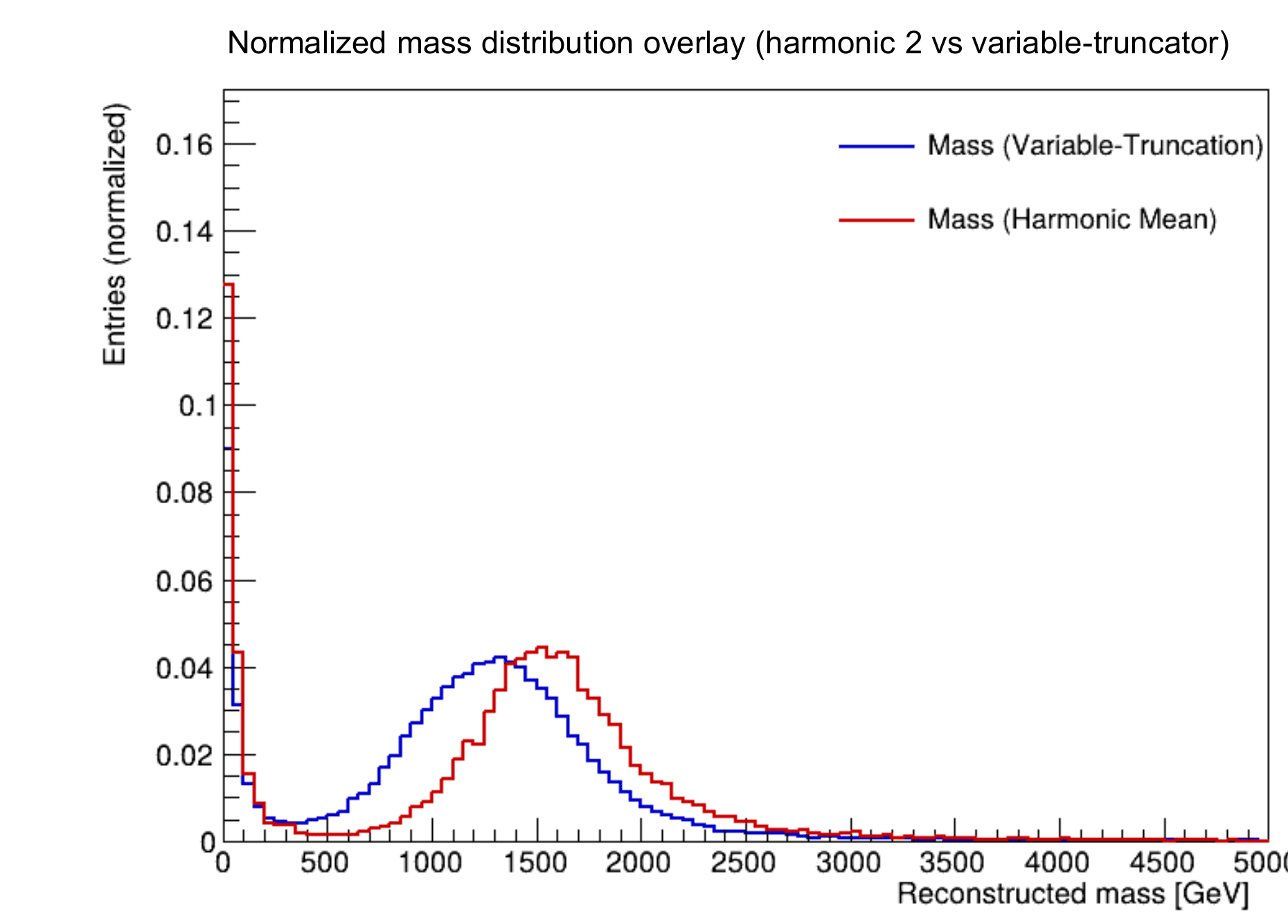
Work carried on past the summer, and that is where the adaptive truncation came from: trim each track until what remains looks symmetric, then stop. Against Harmonic-2 the peak sits a little lower, and the distribution is tighter.
Most of the fall, though, went into the ntuplizer for the HSCP end-to-end analysis framework — the code that turns detector data into the tables everything downstream reads.